エクセル 表の作り方

はじめに

エクセルの表の作り方を紹介します。

初めて表を作成する人向けに、表の作り方の基本を一から紹介します。

見出しやデータの入力、背景色と文字色の設定、罫線の引き方、フィルタや集計方法などを紹介します。

完成例

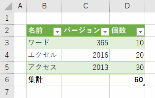
次のような表を作成します。

[ホーム] タブをクリックし、スタイルグループにある [テーブルとして書式設定] をクリックすれば一発で完成します。

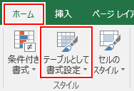
この機能を使用しないで手動で作成する手順を紹介します。手動で作成できるようになると、自由に表をカスタマイズできるようになります。

見出しを作成する

[見出し] を入力します。

[見出し] を範囲選択します。

[ホーム] タブをクリックし、フォントグループにある [太字] をクリックします。

塗りつぶしの色の [▼] をクリックして [背景色] を選択します。

フォントの色の [▼] をクリックして [文字色] を選択します。

見出しが作成されます。

データを作成する

[データ] を入力します。

すべての [セル] を範囲選択します。

[ホーム] タブをクリックし、フォントグループにある罫線の [▼] をクリックして [線の色] から [色] を選択します。

続けて、罫線の [▼] をクリックして [格子] をクリックします。

データと罫線が作成されます。

フィルタ機能を追加する

表の [セル] を 1 つ選択します。

[データ] タブをクリックし、並べ替えとフィルターグループにある [フィルター] をクリックします。

見出し行にフィルターボタンが表示されます。[▼] をクリックして並べ替えや絞り込みができるようになります。

名前の「エクセル」で絞り込むと、このような表示になります。

集計行を作成する

1 番下の [行] を範囲選択します。

[ホーム] タブをクリックし、フォントグループにある格子の [▼] から [下二重罫線] をクリックします。

[集計] を入力します。

[集計行] を範囲選択します。

[ホーム] タブをクリックし、フォントグループにある [太字] をクリックします。

合計などの集計結果を表示する [セル] を選択します。

[数式] タブをクリックし、関数ライブラリグループにある [オートSUM] から [集計方法] を選択します。ここでは [合計] を選択します。

Enter キーを入力します。

個数の合計を求められます。

フィルタ機能を使用するとき

集計結果はフィルタで非表示にしているセルの値も含まれます。

これを表示されているセルのみで集計するには「SUBTOTAL 関数」を使用します。

表示されている個数の合計を求められます。